SSTable

SSTable is an abbreviation for Sorted String Table. It is the fundamental storage building block in few of the modern Log Structured Merge Tree(LSM) based distributed database systems and key-value stores. It is used in Cassandra, BigTable and other systems. SSTable stands for Sorted Strings Table which stores a set of immutable row fragments or partitions in sorted order based on row/partition keys. This article explains how the open source Cassandra defines the format of SSTable. Using the information in this article you can understand implementation of SSTable in other systems.

 

Cassandra creates a new SSTable when the data of a column family in Memtable is flushed to disk. SSTable files of a column family are stored in its respective column family directory. This article describes the format used for Thrift column family. Please check the latest post New Storage Format for the storage format changes in Cassandra 3.0 and the CQL Storage format post to understand how CQL Tables are stored in Cassandra 2.0.


The data in a SSTable is organized in six types of component files.  The format of a SSTable component file is
<keyspace>-<column family>-[tmp marker]-<version>-<generation>-<component>.db

<keyspace> and <column family> fields represent the Keyspace and column family of the SSTable, <version> is an alphabetic string which represents SSTable storage format version, <generation> is an index number which is incremented every time a new SSTable is created for a column family and <component> represents the type of information stored in the file. The optional "tmp" marker in the file name indicates that the file is still being created. The six SSTable components are Data, Index, Filter, Summary, CompressionInfo and Statistics.

For example, I created a column family data in Keyspace usertable using cassandra-cli and inserted 1000 rows {user0, user1,...user999} with Cassandra version 1.2.5.

create keyspace usertable with placement_strategy = 'org.apache.cassandra.locator.SimpleStrategy' and strategy_options = {replication_factor:1};
use usertable;
create column family data with comparator=UTF8Type;

The SSTables under cassandra/data/usertable/data directory:

usertable-data-ic-1-CompressionInfo.db
usertable-data-ic-1-Data.db
usertable-data-ic-1-Filter.db
usertable-data-ic-1-Index.db
usertable-data-ic-1-Statistics.db
usertable-data-ic-1-Summary.db
usertable-data-ic-1-TOC.txt

In the above SSTable listing, the SSTable storage format version is ic, generation number is 1. The usertable-data-ic-1-TOC.txt contains the list of components for the SSTable.

Data file stores the base data of SSTable which contains the set of rows and their columns. For each row, it stores the row key, data size, column names bloom filter, columns index, row level tombstone information, column count, and the list of columns.  The columns are stored in sorted order by their names. Filter file stores the row keys bloom filter.

Index file contains the SSTable Index which maps row keys to their respective offsets in the Data file. Row keys are stored in sorted order based on their tokens. Each row key is associated with an index entry which includes the position in the Data file where its data is stored. New versions of SSTable (version "ia" and above), promoted additional row level information from Data file to the index entry to improve performance for wide rows. A row's columns index, and its tombstone information are also included in its index entry. SSTable version "ic" also stores column names bloom filter in the index entry.



Summary file contains the index summary and index boundaries of the SSTable index. The index summary is calculated from SSTable index. It samples row indexes that are index_interval (Default index_interval is 128) apart with their respective positions in the index file. Index boundaries include the start and end row keys in the SSTable index.

CompressionInfo file stores compression metadata information that includes uncompressed data length, chuck size, and a list of the chunk offsets. Statistics file contains metadata for a SSTable. The metadata includes histograms for estimated row size and estimated column count. It also includes the partitioner used for distributing the key, the ratio of compressed data to uncompressed data and the list of SSTable generation numbers from which this SSTable is compacted. If a SSTable is created from Memtable flush then  the list of ancestor generation numbers will be empty.

All SSTable storage format versions and their respective Cassandra versions are described in https://github.com/apache/cassandra/blob/trunk/src/java/org/apache/cassandra/io/sstable/Descriptor.java and the different components are described in https://github.com/apache/cassandra/blob/trunk/src/java/org/apache/cassandra/io/sstable/Component.java

SSTable data format (version "jb")

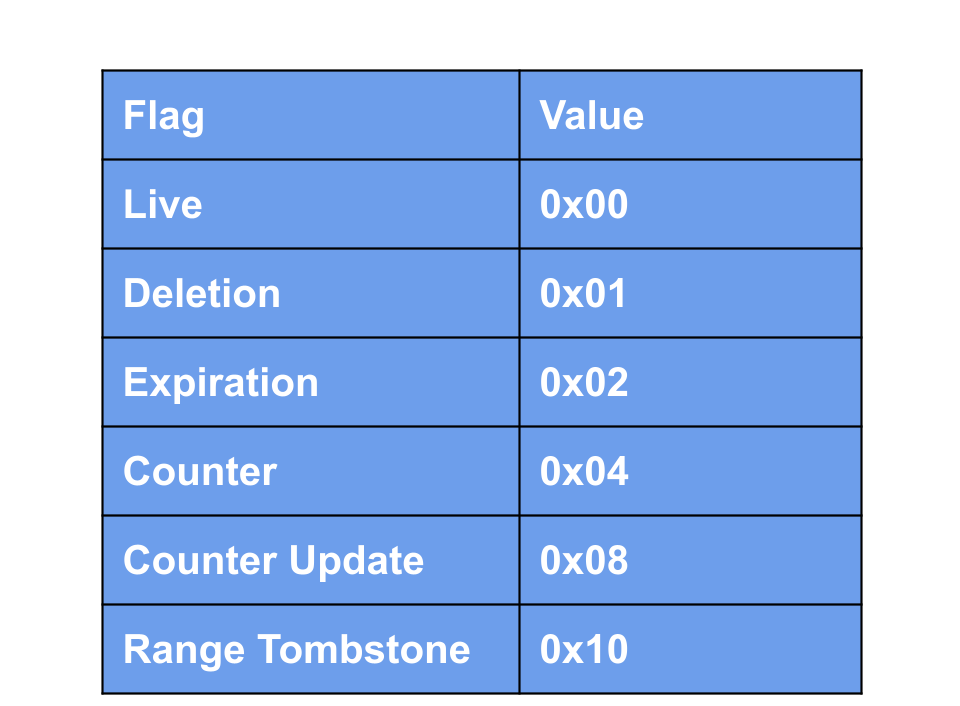
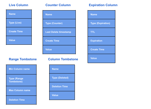
A column inside a row is stored as four parts. It begins with column name, followed by the type of the column, its creation time and column value. A column name is stored as two bytes indicating the length of the name followed by the name itself. The type is a one byte mask value indicating the type of stored column. Based on the column type remaining bytes of the column are processed.

Column timestamp is a eight bytes value indicating the column creation time. For a deleted column, the timestamp indicated the time when the column was deleted. Column value is stored as four bytes indicating the value size followed by the bytes storing the actual column value.

Version "ja"

In version "ja" SSTable format, Column names bloom filter, Column count fields  are removed from SSTable data component file. The fields, localDeletionTime and  markedForDeleteAt added to represent deletion timestamps of a row. For a row tombstone, localDeletionTime represents the  timestamp in seconds at which a top level tombstone is created and markedForDeleteAt represents a timestamp in microseconds after which the data in a row should be considered as deleted. The default value for localDeletionTime is 0x7fffffff and the default value for markedForDeleteAt is 0x8000000000000000. If a row's deletion timestamps contain the default values then it contains live data.

Row size field is also removed from data component file. A special 0 length column name is added to represent the end of row. Row size is calculated from Index file. Index file contains starting offsets of each row.  Successive offsets are used to calculate each row size except for the last row in SSTable. For the last row, end of data file is used to calculate its size.

Version "ka"

In version "ka", contents of Statistics component file is split in to 3 types of metadata called validation, compaction and stats. Validation metadata is used to validate SSTable which includes partitioner and bloom filter fp chance fields. Compaction metadata includes ancestors information which is also available in older formats and a new field called cardinality estimator. Cardinality estimator is used to efficiently pre-allocate bloom filter space in a merged compaction file by estimating how much the input SStables overlap. Stats metadata contains rest of the information available in old formats and two additional fields. First one is a flag to track the presence of local/remote counter shards and the other one is for storing the repair time.
 
sstable2json.py

sstable2json.py reads the rows and columns in a given SSTable and converts those to JSON format similar to sstable2json tool available in Cassandra distribution. It doesn't require access to Cassandra column families in system keyspace to decode SSTable data like sstable2json tool. It is tested with version "jb".

Other two important components of Cassandra storage architecture are Memtable and CommitLog which are described in following blog posts.

 

Cassandra Memtable

Cassandra CommitLog 

Using Merkle trees to detect inconsistencies in data

Cassandra's AntiEntropy service uses Merkle trees to detect the inconsistencies in data between replicas. Merkle tree is a hash tree where leaves contain hashes of individual data blocks and parent nodes contain hashes of their respective children. It provides an efficient way to find differences in data blocks stored on replicas and reduces the amount of data transferred to compare the data blocks.

Cassandra's implementation of Merkle tree (org.apache.cassandra.utils.MerkleTree) uses perfect binary tree where each leaf contains the hash of a row value and each parent node contains hash of its right and left child. In a perfect binary tree all the leaves are at the same level or at same depth. A perfect binary tree of depth h contains 2^h leaves. In other terms if a range contains n tokens then the Merkle tree representing it contains log(n) levels.

When nodetool repair command is executed, the target node specified with -h option in the command, coordinates the repair of each column family in each keyspace. A repair coordinator node requests Merkle tree from each replica for a specific token range to compare them. Each replica builds a Merkle tree by scanning the data stored locally in the requested token range. The repair coordinator node compares the Merkle trees and finds all the sub token ranges that differ between the replicas and repairs data in those ranges.

A replica node builds a Merkle tree for each column family to represent hashes of rows in a given token range. A token range can contain up to 2^127 tokens when RandomPartitioner is used. Merkle tree of depth 127 is required which contains 2^127 leaves. Cassandra builds a compact version of Merkle tree of depth 15 to reduce the memory usage to store the tree and to minimize the amount of data required to transfer Merkle tree to another node. It expands the tree until a given token range is split in to 32768 sub ranges. In the compact version of tree, each leaf represents hash of all rows in its respective sub range. Regardless of their size and split, two Merkle trees can be compared if they have same hash depth.

For example, the token range (0, 256], contains 256 sub ranges (0, 1], (1, 2]...(255, 256] each containing single token. A perfect binary tree of depth 8 is required to store all 256 sub range hashes at leaves. A compact version of tree with depth 3 for the same range contains only 8 leaves representing hashes of sub ranges (0, 32], (32, 64] ... (224, 256] each containing 32 tokens. Each leaf hash in this compact version of tree is a computed hash of all the nodes under it in the perfect binary tree of depth 8.

Building Merkle tree with RandomPartitioner

RandomPartitioner distributes keys uniformly , so the Merkle tree is constructed recursively by splitting the given token range in to two equal sub ranges until maximum number of sub ranges are reached. A root node is added with the given token range (left, right] and the range is split in to two halves at a token which is at the midpoint of the range. A left child node is added with range (left, midpoint] and a right child node is added with range covering (midpoint, right]. The process is repeated until required number of leaves (sub ranges) added to the tree. 

Next row hashes are added to the Merkle tree in sorted order. Each row's hash value is computed by calculating MD5 digest of row value which includes row's column count, column names and column values but not the row key and row size. The deleted rows (tombstones) hashes are also added to the tree which include the delete timestamps. Row hashes are added to Merkle tree leaves based on their tokens. If a leaf's sub range contains multiple rows, its hash is computed by combining hashes of all rows covered by its range using XOR operation. Non leaf nodes hashes are computed by performing XOR on hashes of their respective children.

Comparing Merkle trees

Two Merkle trees are compared if both of them cover the same token range regardless of their size. The trees are compared recursively starting at root hash. If root hashes match in both the trees then all the data blocks in the tree's token range are consistent between replicas.  If  root hashes disagree, then the left child hashes are compared followed next by right child hashes. The comparison proceeds until all the token ranges that differ between the two trees are calculated.

Sample Java code to test Merkle tree

import java.util.*;
import org.apache.cassandra.dht.*;
import org.apache.cassandra.utils.*;
import org.apache.cassandra.utils.MerkleTree.RowHash;
import org.apache.cassandra.utils.MerkleTree.TreeRange;
import org.apache.cassandra.utils.MerkleTree.TreeRangeIterator;
import static org.apache.cassandra.utils.MerkleTree.RECOMMENDED_DEPTH;

public class MerkleTreeTest {

    public static void addRows(MerkleTree tree, Map<BigIntegerToken, byte[]> rows) {
        MerkleTree.RowHash EMPTY_ROW = new MerkleTree.RowHash(null, new byte[0]);

        // Get the sub range iterator which iterates over sorted sub ranges
        TreeRangeIterator ranges = tree.invalids();
        TreeRange range = ranges.next();

        for (BigIntegerToken token : rows.keySet()) {
            while (!range.contains(token)) {
                // add the empty hash, and move to the next range
                range.addHash(EMPTY_ROW);
                range = ranges.next();
            }
            range.addHash(new RowHash(token, rows.get(token)));
        }
        if (range != null) {
            range.addHash(EMPTY_ROW);
        }
        while (ranges.hasNext()) {
            range = ranges.next();
            range.addHash(EMPTY_ROW);
        }
    }

    public static void main(final String[] args) {

        // Sorted map of hash values of rows
        Map<BigIntegerToken, byte[]> rows1 = new TreeMap<BigIntegerToken, byte[]>();
        rows1.put(new BigIntegerToken("5"), new byte[] { (byte)0x09 });
        rows1.put(new BigIntegerToken("135"), new byte[] { (byte)0x0c });
        rows1.put(new BigIntegerToken("170"), new byte[] { (byte)0x05 });
        rows1.put(new BigIntegerToken("185"), new byte[] { (byte)0x02 });

        Map<BigIntegerToken, byte[]> rows2 = new TreeMap<BigIntegerToken, byte[]>();
        rows2.put(new BigIntegerToken("90"), new byte[] { (byte)0x03 });
        rows2.put(new BigIntegerToken("135"), new byte[] { (byte)0x0c });
        rows2.put(new BigIntegerToken("170"), new byte[] { (byte)0x05 });
        rows2.put(new BigIntegerToken("185"), new byte[] { (byte)0x02 });

        // Create Merkle tree of depth 3 for the token range (0 - 256]
        IPartitioner partitioner = new RandomPartitioner();
        Range fullRange = new Range(new BigIntegerToken("0"), new BigIntegerToken("256"), partitioner);
        MerkleTree tree1 = new MerkleTree(partitioner, fullRange, RECOMMENDED_DEPTH, 8);
        tree1.init();
        MerkleTree tree2 = new MerkleTree(partitioner, fullRange, RECOMMENDED_DEPTH, 8);
        tree2.init();

        // Add row hashes
        addRows(tree1, rows1);
        addRows(tree2, rows2);

        // Calculate hashes of non leaf nodes
        List<TreeRange> diff = MerkleTree.difference(tree1, tree2);
        System.out.println("tree1: " + tree1);
        System.out.println("tree2: " + tree2);
        System.out.println("difference: " + diff);
    }
}

Output:

tree1: #<MerkleTree root=#<Inner 128 hash=[02] children=[#<Inner 64 hash=[09] children=[#<Inner 32 hash=[09] children=[#<Leaf [09]> #<Leaf []>]> #<Inner 96 hash=[] children=[#<Leaf []> #<Leaf []>]>]> #<Inner 192 hash=[0b] children=[#<Inner 160 hash=[0b] children=[#<Leaf [0c]> #<Leaf [07]>]> #<Inner 224 hash=[] children=[#<Leaf []> #<Leaf []>]>]>]>>

tree2: #<MerkleTree root=#<Inner 128 hash=[08] children=[#<Inner 64 hash=[03] children=[#<Inner 32 hash=[] children=[#<Leaf []> #<Leaf []>]> #<Inner 96 hash=[03] children=[#<Leaf [03]> #<Leaf []>]>]> #<Inner 192 hash=[0b] children=[#<Inner 160 hash=[0b] children=[#<Leaf [0c]> #<Leaf [07]>]> #<Inner 224 hash=[] children=[#<Leaf []> #<Leaf []>]>]>]>>

difference: [#<TreeRange (0,32] depth=3>, #<TreeRange (64,96] depth=3>]

References:

http://en.wikipedia.org/wiki/Merkle_tree
http://wiki.apache.org/cassandra/AntiEntropy
https://github.com/apache/cassandra/blob/trunk/src/java/org/apache/cassandra/utils/MerkleTree.java

key to token with random partitioner

Cassandra supports various strategies to partition data across nodes in a cluster. User can choose available strategies as required by an application. Most commonly used strategy is to evenly distribute keys across the nodes using consistency hashing scheme.

In Cassandra, data is stored in rows in column families on nodes. Each row is identifiedby a unique key. The nodes in a cluster are formed as a ring where each node is assigned with a fixed position on the ring represented by a token and is responsible to store a range of keys.Each row key is also mapped to a token and assigned to nodes based on the token position in the token space.

The default Partitioner is RandomPartitioner (org.apache.cassandra.dht.RandomPartitioner) which uses MD5 hashing algorithm to map keys to tokens. It uses unsigned big integer of length 128 bits to represent a token and the possible token space consists of tokens from 0 to 2^127-1.

A key is converted to token by calculating MD5 digest of the contents of the key and the resulted digest is converted to hexadecimal format and represented in 2's complement form. Here is the python code to map a key to token

gettoken.py:

import hashlib

key = "foo"

# Calculate MD5 digest and convert it to hex format
digest = hashlib.md5(key).hexdigest()

# Convert the hash digest to 2's complement form
token  = long(digest, 16)
bits   = 128
if ((token & (1 << (bits - 1))) != 0):
    token = token - (1 << bits)

# Convert the resulting number to unsigned form
print abs(token)

$ python token.py
110673303387115207421586718101067225896

You can checkout the code at github ctools